Visual Concept Learning on Fashion-MNIST

I trained a Deep Belief Network on Fashion-MNIST without labels, then probed what each of its three layers had learned and how it breaks. The most interesting result: the same model that collapses under random noise holds up far better than a standard neural network under a targeted adversarial attack.

This was my individual project for Cognition and Computation at the University of Padova, taught by Prof. Marco Zorzi and Dr. Alberto Testolin. It was graded 10/10, with the feedback “very good and thorough work”.

The brief was to simulate computational models of visual concept learning and analyze them along four axes: what each layer of the hierarchy represents, how the model’s internal representations are organized, what kind of errors it makes, and how it reacts to adversarial attacks. The deliverable was a single self-contained Jupyter notebook, with the reasoning written next to the code.

The central hypothesis: a hierarchical model trained without labels should build representations that become more abstract and easier to separate as you go deeper. I turned that into four questions:

1. Do deeper layers make the classes more linearly separable?
2. What does each layer actually encode, and do similar garments end up close together?
3. Which errors does the model make, and how does it degrade as the input gets noisier?
4. How vulnerable is it to adversarial perturbations, and can its generative structure be used as a defense?

The aim was not the highest possible accuracy, but understanding how the model organizes visual concepts and where that organization breaks.

I used Fashion-MNIST: 70,000 grayscale 28×28 images of clothing in 10 classes. I picked it because several classes genuinely overlap (shirt, pullover, coat), which makes the errors worth studying.

Component	Role	Details
Deep Belief Network	Main model, trained without labels	3 stacked RBMs, 400 → 500 → 800 units, contrastive divergence (CD-1)
Linear read-outs	Probe each layer (H1, H2, H3)	One linear classifier per layer; if a linear model separates the classes, the layer has done the work
Feed-forward network	Supervised baseline	Same hidden sizes, trained end-to-end with labels

Model selection

I kept tuning deliberately small and repeatable rather than exhaustive. For the DBN I first compared CD-1 against CD-3 on a held-out validation split: they matched (about 76.7% on H3), so CD-1 won on cost. A later round compared four variants per model (learning rate, width, CD steps) over 3 seeds, ranking them on clean, noisy and adversarial accuracy together, with mean, standard deviation and 95% confidence intervals. The baseline configurations stayed the best overall compromise for both models.

Stress tests

• Random noise: additive Gaussian noise of increasing strength, clipped to valid pixel values, averaged over 5 runs per level.
• Adversarial attack: the Fast Gradient Sign Method (FGSM) nudges every pixel by a small amount ε in the direction that most increases the model’s loss. I ran it untargeted on the full test set, plus a targeted demo steering samples towards “bag”.
• Defense: before classifying, pass the input up and back down the DBN once or twice, so the model reconstructs a cleaner version of the image.

The middle layer is the sweet spot

Depth helped, but not all the way down. H2 gave the best linear read-out and the most compact clusters; H3 pushed classes further apart while spreading each class out.

Layer	Linear read-out accuracy	Silhouette score	Inter/intra-class distance
H1 (400 units)	82.51%	0.044	0.96
H2 (500 units)	82.92%	0.061	1.01
H3 (800 units)	82.86%	0.049	1.22

The receptive fields tell the same story. H1 learns local strokes: contours, hems, the central area of a garment. H2 and H3, projected back into pixel space, combine them into more global, garment-shaped templates.

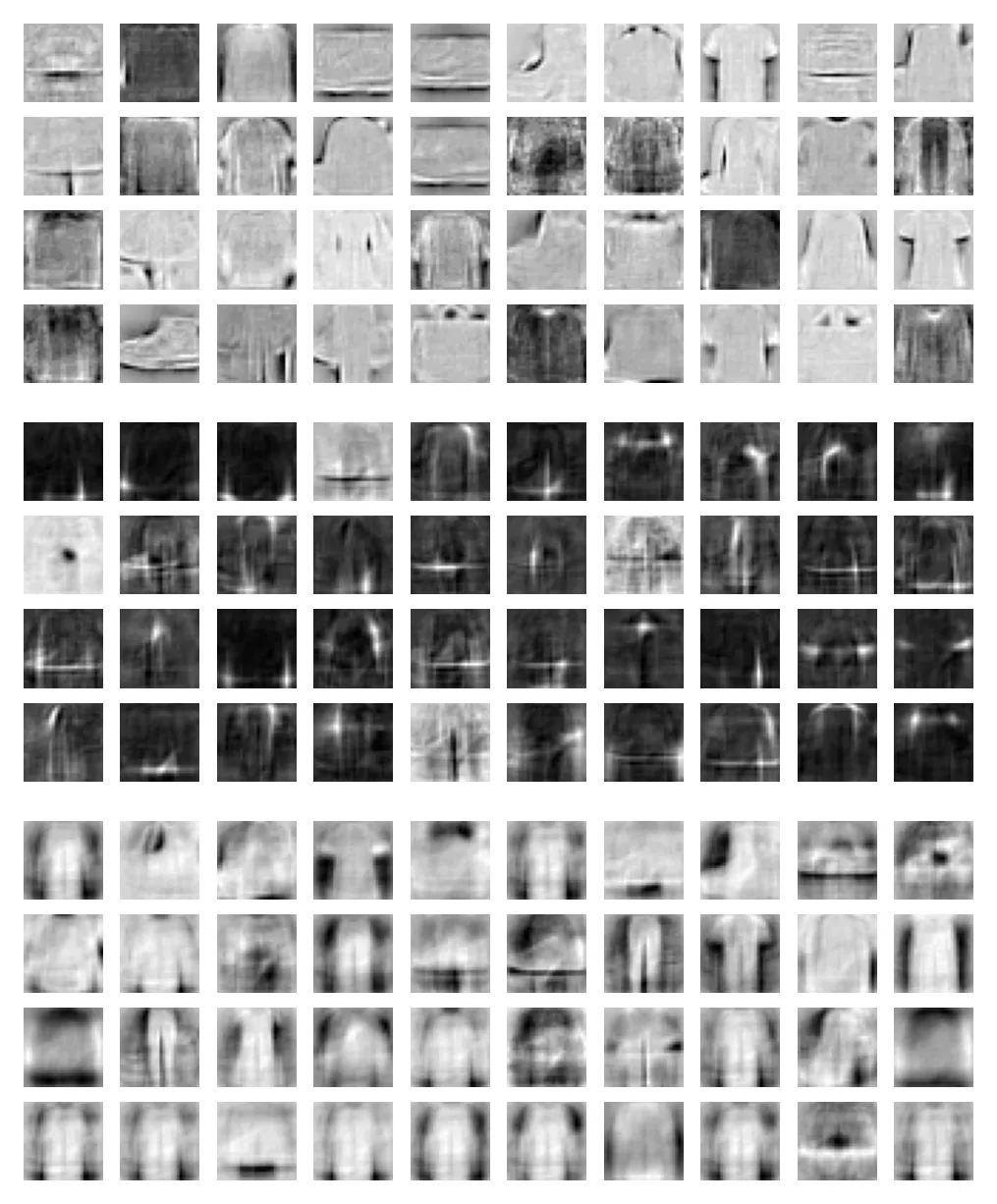
Receptive fields of the first 40 units of each layer, projected into pixel space. Top to bottom: H1, H2, H3.

Clustering the average activation of each class gives plausible pairs at every layer: sandal with sneaker, pullover with shirt, while bag stays apart from the wearable items. Depth refines this structure rather than inventing a new one.

One check I’m glad I ran: some H3 filters looked “dead” in the plots. Varying the display threshold showed this was mostly a visualization artifact (at threshold 0.1 only 72% of H3 weights survive, at 0.05 over 99% do), not a property of the model.

Same accuracy, different mistakes

On clean test images the DBN read-outs edge out the supervised baseline (82.9% for H2 against 82.1%), but the confusion matrices show very different errors. Both struggle with pullover, coat and shirt. The DBN read-outs get shirts right about 53% of the time; the feed-forward network only 30%, scattering the rest almost evenly across T-shirt, pullover and coat.

Under Gaussian noise the DBN loses clearly. At σ = 0.4 the feed-forward network still scores about 71%, while the read-outs drop to 14–27%. They reach chance level (10%) around σ = 0.6–0.7, H3 first; the feed-forward network stays above chance even at σ = 2.0.

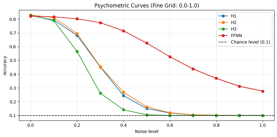
Accuracy as Gaussian noise increases. The read-outs fall to chance around σ = 0.6–0.7; the feed-forward network degrades much more slowly.

Under attack, the ranking flips

Against FGSM the DBN degrades gradually, while the supervised network collapses almost immediately:

Attack strength ε	Feed-forward network	DBN + read-out
0.00	~82%	~81%
0.05	~50%	~65%
0.10	~18%	~40%
0.20	0.8%	12.3%

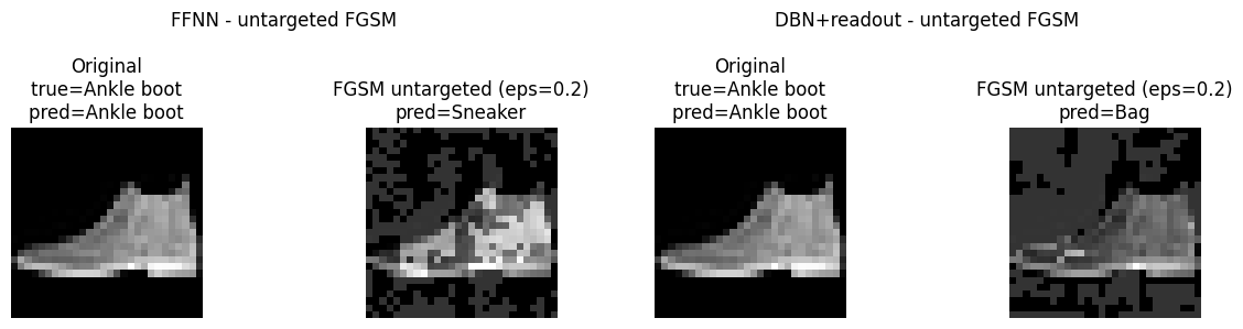
One test image under untargeted FGSM at ε = 0.2. At this strength both models are fooled; the difference shows over the whole test set.

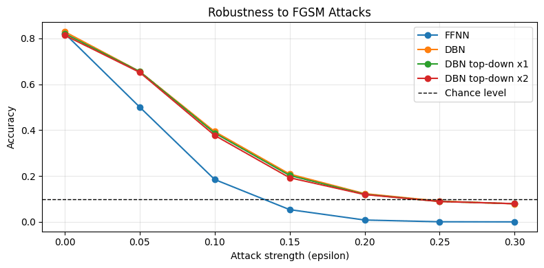
Accuracy against attack strength. The two reconstruction-defense curves sit on top of the undefended DBN.

The reconstruction defense did not help: its curves sit on top of the undefended DBN (12.1% vs 12.3% at ε = 0.20).

Robustness is not one property. The same model was the most fragile against random noise and the most resilient against a gradient-based attack, so a single robustness number would have hidden half the picture. The same goes for accuracy: two models within one point of each other made very different mistakes.

Deeper is not automatically better either. The unsupervised hierarchy did produce more abstract features, but the most useful layer for classification was the middle one.

Negative results count. The reconstruction defense had a sound rationale and did nothing measurable here; I’d rather report that than drop it.

Limits

• FGSM is a single-step attack. Iterative attacks such as PGD are stronger and would be the real test of the DBN’s adversarial advantage.
• Tuning was compact, and some tuning-phase adversarial numbers were estimated on a 2,000-image subset.
• The DBN code is downloaded at runtime from an external repository; vendoring it would make the work fully reproducible.

The full notebook, with code, every figure and the complete discussion: Jupyter notebook (3 MB).

Tools: Python, PyTorch, torchvision, scikit-learn, matplotlib.